Modernizing Risk Analysis
By Joan C. Barrett
Risk Management, February 2025

Actuaries are the premier risk analysts in the world. At least for now. The problem is, the nature of risk is changing quickly, decision-makers are expecting more insightful analytics, and new analytical techniques, like artificial intelligence (AI) are being developed at a rapid pace. We have to keep pace. An important step in that direction is to incorporate total risk analysis (TRA) into our day-to-day work.
About TRA
Why TRA? Picture this. You are in a meeting with your boss. You have just presented your recommendation for next year’s budget. Your boss was smiling and nodding during the whole presentation. You are really proud of yourself. Then, the boss asks the question, “What are the chances we will go over budget by more than $1 million?” How do you answer that question? Do you start by saying “it depends,” followed by a list of things that could go wrong or can you confidently say “15%”? TRA is a framework for consistently answering questions like this.
As it turns out, TRA is the logical next step in the analytics we have been doing for years. There are two important extensions to that analysis, however. The first is that TRA provides a framework for a more comprehensive view of future risks. Historically, actuaries and others have relied heavily on projecting past experience in their analysis. This will not change, but TRA provides a framework for quantifying emerging risks, like climate change and financial volatility. Second, a key element of TRA is distinguishing between the random variation (RV) risk and the projection risk. Many current analytics conflate the two, making it difficult, if not impossible, to determine if you missed a projection because of the things you could control, the model design and choice of parameters, or because of things you cannot control, the RV risk.
For more information about TRA, read the paper “Calculated Risk: Driving Decisions Using the 5/50 Research,”[1] as it describes the concepts discussed below in more detail.
A TRA Example
Perhaps, the easiest way to explain the theory behind TRA is to use the classic coin-flip analogy. Before we begin the example, some terminology. As noted above, TRA distinguishes between two innate types of risks: The RV risk and the projection risk. Suppose you are given a coin you know is fair. You may know this because the coin has already been flipped thousands of times and/or because you know how the coin was manufactured. If that is the case, you can confidently place bets assuming the probability of heads is 50%. This is the RV risk. But what if it is a new type of coin, one that you are not familiar with, one that looks like it may not be a fair coin? If that is the case, then you have to consider the fact that the probability of heads may not be 50%. That is the projection risk. Applying these principles requires the 4-step process shown in Figure 1.
Figure 1
The TRA Process
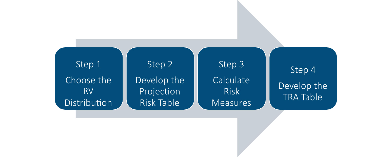
If you are only making one bet, Step 1 is easy. It is the binomial distribution with the mean equal to the probability of heads, p, and a variance of p x (1 – p). In this example, however, you will be making 100 bets. This means that the normal distribution can be used as an approximation. The formula for the mean is N x p and the variance is N x p x (1 -p), where N is the number of coin flips. In our example, if the coin is fair, then the mean is 50 (100 x 0.5) and the variance is 25 x (100 x 0.5 x 0.5). Of course, if the variance is 25, then the standard deviation is the square root of the variance or 5.0.
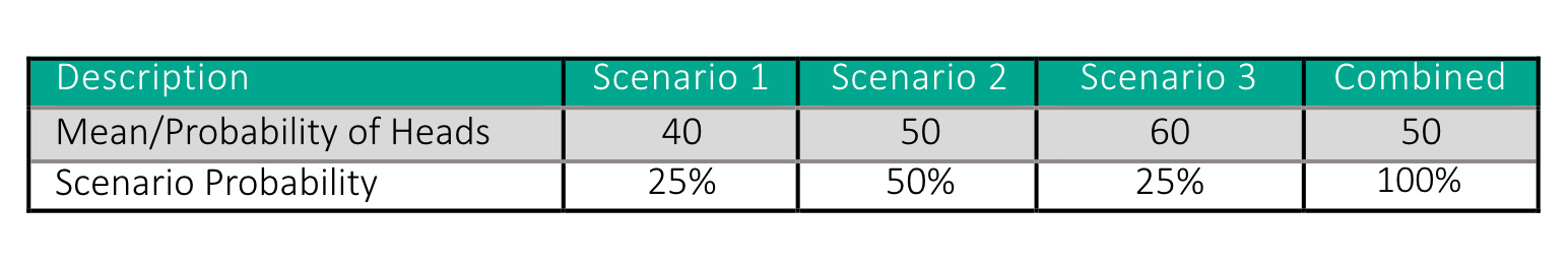
The goal of Step 2 is to create a table like Table 1. Theoretically, the projection risk table should include every possible value of p and the associated probability for that value. In this example, and in many real-life situations, scenarios are used to make the calculations easier to produce and to explain. Assigning probabilities to each scenario may require both a quantitative and qualitative analyses. An example of a quantitative analysis would be to test the coin for, say, 10 flips. The qualitative analysis may be as simple as a guess or it may be based on looking at the coin or how the coin feels in your hand. The probabilities in Table 1 are purely hypothetical and chosen for illustrative purposes only.
Table 1
The Projection Table
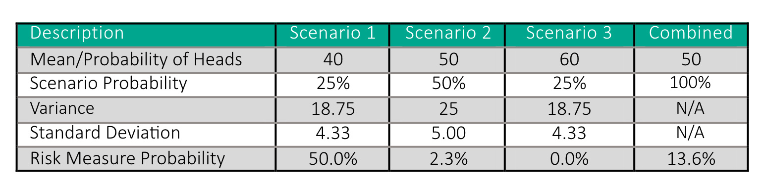
In any financial decision, there are always several ways to measure risk: What is the expected gain/loss? What are the chances I will lose more than my risk tolerance? What are the chances I will break even? In this example, the risk measure is based on the risk tolerance. Specifically, “what are the chances there will be 40 or fewer heads during the 100 flips?” Of course, the answer to that depends on the probability of heads (the mean). If the probability of heads for that coin is 40%, then the chances of having 40 or fewer flips is 50%. If the probability of heads is 50%, then there is a small chance of having fewer than 40 heads since 40 is over two standard deviations from the mean. The final step is to combine these steps into a single table as shown in Table 2. The total risk is simply the weighted average of the risk measure. In this case, the answer is 13.6%.
Table 2
The Total Risk Table
Real-World Examples
Although coin-flip examples are a good way to start, the real world is a little more complicated. Take mortality projections, for example. A mortality projection is similar to the coin-flip example, except that instead of successive flips, mortality is measured over time. The main difference is that the projection table changes over time due to factors like the aging of the population and climate change. This could mean that the best way to analyze the risk is using scenarios that reflect those changing conditions. A technique known as a scenario generator may simplify that process.
In one sense, health care projections are simpler than mortality projections because most of the time the goal is to just project costs for the next year. There are two important differences, however. First, the average year-over-year costs tend to be volatile, as shown in Figure 2. At a national level, some of the factors influencing these results included the 2008 financial crisis and the passage of the Affordable Care Act in 2010. In addition to that uncertainty, health plan sponsors had to examine the impact of internal changes like changes in clinical policies, shifting demographics, and negotiations with providers.
Figure 2
National Health Care Expenditures
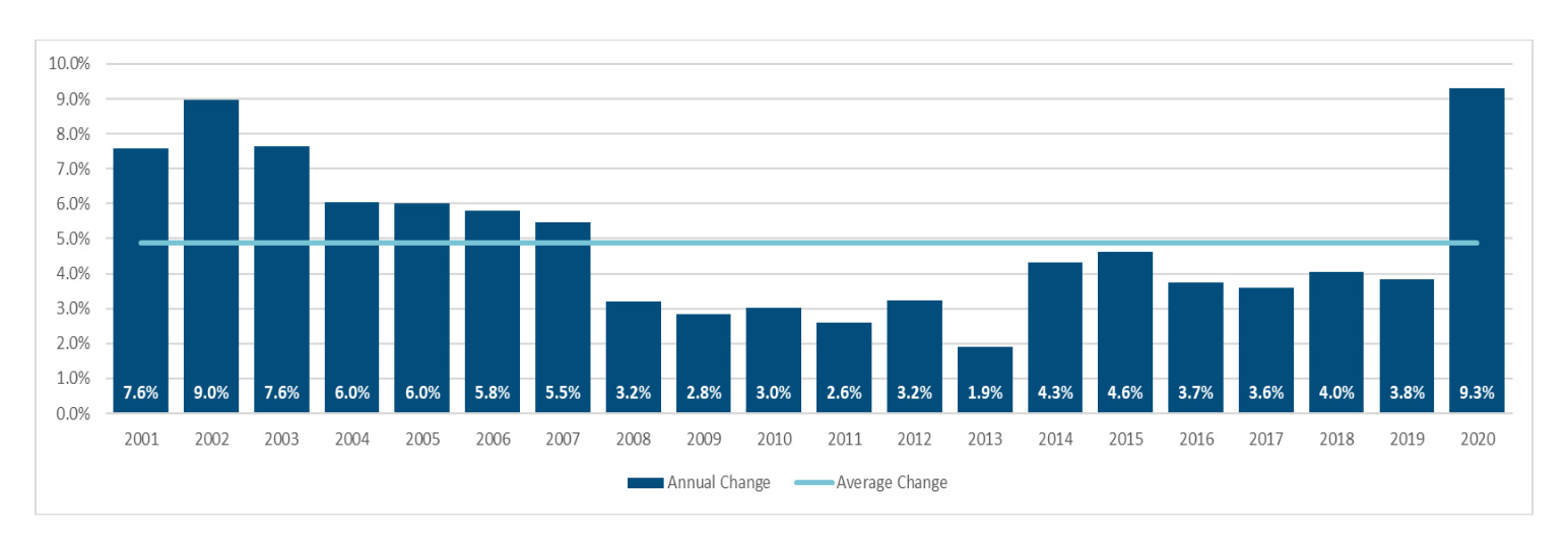
Source: Centers for Medicare and Medicaid Services. 2023. Historical National Health Expenditures, Table 1. CMS.gov, https://www.cms.gov/data-research/statistics-trends-and-reports/national-health-expenditure-data/historical (accessed Sept. 15, 2023).
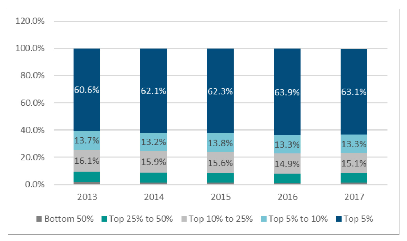
The other major difference is that the binomial distribution does not apply. Instead, the appropriate distribution is the cost distribution like the ones shown in Figure 3. As the name implies, a cost distribution is simply the distribution of costs for a given time period, such as a calendar year. Figure 3 shows that the distribution of costs is consistent from year to year, although the average cost per person varies considerably as indicated in Figure 3. This means that the RV risk can be quantified using a cost distribution and the projection risk can be quantified by examining the variance associated with projecting the average cost per person.
Figure 3
Commercial Insurance Cost Distributions
Where Do We Go from Here?
In my mind, the goal is for the concept of TRA to eventually be included in every practice area regardless of the underlying analytical techniques used in the projection process. To make this happen will require a combination of education and research. This article is one of many efforts to promote the TRA concept. Other avenues include webinars, meeting sessions, and discussion groups within the SOA.
Research efforts will take time. There are two primary areas of interest. The first is to gain a better understanding of emerging risks. According to the latest Emerging Risk Survey,[2] the top emerging risks include climate change, wars (including civil wars), disruptive technology, shifting demographics, and cyber-attacks. Some of these risks, like climate change shifting demographics, impact businesses on a daily basis and should be incorporated into pricing and other analytics as appropriate. Other risks, like cyber-attacks, are more event-driven and should be incorporated into enterprise risk management analytics. In all likelihood, this type of research will be led by practicing actuaries with a goal of better understanding the nature of the risk, the applicability to a specific practice area, and techniques for quantifying the risks.
The other area for research is expanding the underlying analytics. The purpose of the Calculated Risk paper was to describe the TRA process for health care. To keep things simple, the paper simply described some thoughts on how to manage the underlying analytical techniques. In particular, more work needs to be done in developing techniques to separate the RV risk from the projection risk and to find ways to estimate the variance for more sophisticated projection techniques, especially machine learning techniques.
Statements of fact and opinions expressed herein are those of the individual authors and are not necessarily those of the Society of Actuaries, the newsletter editors, or the respective authors’ employers.
Joan C. Barrett, FSA, MAAA, is a partner at Axene Health Partners, LLC. She can be contacted at joan.barrett@axenehp.com.
Endnotes
[1] Barret, Joan, Natsis, Achilles, Pistilli, Tony. “Calculated Risk: Driving Decisions Using the 5/50 Research.” Society of Actuaries. 2024. Calculated Risk: Driving Decisions Using the 5/50 Research | SOA
[2] Rudolph, Max J., 17th “Annual Survey of Emerging Risks,” 2024. Society of Actuaries. 17th Annual Survey of Emerging Risks | SOA