Challenges of Managing Interest Rate Risk: Part 6—How to get the Most Insight out of a Company's Assets and Liabilities
By Dariush Akhtari
Risk Management, February 2025
Editor’s note: The author extends heartfelt gratitude to Michel Perrin for his unwavering dedication, investing countless hours in thoughtful review, insightful discussions, and meticulous analysis of the various approaches. His expertise, patience, and collaborative spirit were invaluable to this endeavor, and his contributions significantly enhanced the quality and depth of this work.

In this part, I will show that the rates to be shifted in the key-rate calculation are forwards and not spots. This is due to the fact that most cash flows being discounted in the value calculation are dependent on the forward rates. I will show that if spots are shifted up/down, they would not necessarily result in forwards being up/down for all the years in the particular key rate, resulting in unexpected results. I will further show how metrics calculated by shifting forwards versus spots enhance the accuracy of the approximation of projected value in various rate environments. In the next and final part of this series, I’ll introduce two approaches in approximating change in value that do not rely on the ALM metrics discussed so far.
Forward Rate versus Spot Rate
In the calculation of ALM metrics, many shift the spot or par rates. When this shift is applied to the entire curve, the shift to the forward is within a very small fraction of the shift in the spot. I believe that the practice in the industry (which I, too, have applied in the past and in the examples provided in the prior part) has inadvertently become to also shift the spots in the calculation of key rates, whereas it should have been to the forward. However, the shift to the rate needs to be fit for the purpose. Most insurance products use a crediting rate that is dependent on the earned rate of the portfolio of assets backing them. In the projection models, these earned rates are akin to forward rates as they represent the earned rate for the period. In the calculation of ALM metrics, rates are shifted up and down and one would expect that when rates are shifted up, the earned rates would be increased and vice versa when rates are shifted down, the earned rates would decrease. However, this would not be the case for the forwards if spot rates are shifted as highlighted in Appendix 1 (i.e., when spot rates are shifted up for a particular key rate, the forward rates for the periods in the key rate are not necessarily shifted up and vice versa). The test with a simple GIC that credits the policyholder based on the period’s earned rate further verified the above. Thus, I recommend that in the calculation of key-rate metrics, forward rates should be shifted unless the projected cash flows are specifically dependent on the spot or par rates, in which case such rates should be shifted. However, this may be rare in the insurance world
Comparison of Unscaled and Cumulative Approaches under Forward Shift
I decided to test if I can improve my approximations by calculating the ALM metrics using a shift to forward. Since I had decided that the cumulative approach produces more stable and reasonable approximations than parallel or scaled approaches, I will only compare unscaled and cumulative approaches. Additionally, since smaller shift sizes produce more accurate results, I would concentrate on 0.5- to 2-bp shifts. As can be seen in the tables in Appendix 2, a cumulative approach produces a materially close approximation to the unscaled approach (i.e., immaterial differences) but with one-seventh of the runs (using seven key rates). However, these tables very clearly highlight how inaccurate the result of shifting spots would be compared with shifting the forwards.
Additionally, smaller shift sizes (0.5bp to 2 bps) seem to generally produce more accurate approximations. Thus, I recommend using a cumulative approach using 1- or 2-bp shift to the forward.
Decreasing the Number of Key Rates
Historical data show, and many argue, that the forward rate is reasonably flat after year 10. I wanted to examine whether I would lose material accuracy if I reduced the key rates to five key rates from seven by eliminating 15- and 25-year key rates. This would reduce the number of runs by four (10 runs instead of 14), a 29% reduction in runtime. As it can be observed in Appendix 2, no material deterioration of the approximation by decreasing the key rates from seven to five based on the simple product I had tested can be observed. Thus, I recommend testing five versus seven key rates for your portfolio to decide if the reduction of four runs (two key rates combined with up and down shifts) would outweigh the possible level of less accuracy in your approximation for your portfolio.
How to get the Most Insights
Cumulative Key Rates
Calculation of cumulative key rates is less computationally intensive than full unscaled. Their calculations require (1/n)th runs where n is the number of key rates used (e.g., (1/5)th using five key rates and (1/7)th using seven key rates). They are relatively “resilient” compared to full unscaled, i.e., they do not fail by materially larger error amounts than unscaled would. As a result, I recommend using this technique combined with shifting forward rates (unless cash flows are specifically dependent on other rates, such as spot, in which case the spot rates should be shifted) for the calculation of key-rate metrics.
OAS Analysis to Identify Inflection Points
I highly recommend projecting liabilities for 100 bps below to 100 bps above current spot rates by 1 bp increments and calculating ALM metrics (DV01 & CV01) at these rates using deterministic runs. In the calculation of the discounted desired measure (cash flow or profits), one would further add the graded option adjusted spread (OAS) calculated from the three separate OAS calculations at current spot rates less 100 bps, current spot rates, and current spot rates plus 100bps as discussed in Part 2. Examining the ratios of consecutive CV01s would identify at what rate increase there would be an inflection point that may result in the distortion of the approximations.
Rebalancing and Recalculation Need
If rates are close to the inflection points highlighted in the OAS analysis, frequent rebalancing and recalculation may be necessary to ensure staying within a company’s risk appetite. This is due to the fact that the calculated ALM metrics may no longer reflect the current ALM metrics post the inflection points.
Conclusion
To mitigate interest-rate risk, it is imperative to match the characteristics of assets to those of liabilities. Historically, duration matching or duration and convexity matching technique was performed for this purpose. However, these techniques do not make the portfolio immune to non-parallel shifts in the interest rate curve. A better technique is to segment interest rate curve in smaller segments (where rates are more prone to move in parallel) and calculate duration and convexity for these segments (known as key-rate duration and key-rate convexity). These ALM metrics better reflect liability characteristics and can further be used to approximate the impact of value change after rates have moved over time. Regardless of the metrics used, it is important to understand the limitations of these metrics and how they are calculated. I have identified two concerns with current methods of calculating key rates. One, the use of scaling (to capture cross key-rate impact without additional runs) and another shifting the spot rates. I then introduced a new technique, namely cumulative key rate, to better capture the interaction of key rates and further showed that forward rates should be shifted in the calculation of key-rate metrics. I also pointed out that such shifts should be small (1 bp to 2 bps) to better reflect the first and second moments of value change with respect to interest rate. Additionally, one should identify the range of rate changes where these metrics may be relied upon. Should rates move outside of such a reliance range, one should perform additional calculations for the potential need for rebalancing of the portfolio. To identify the range of rate change that these metrics can be relied upon, I suggested the use of the calculation of such metrics over a range of +/-100 bps over the current spot rates combined with the use of OAS to limit the needed runtime. I further provided a technique on how to use these runs to improve the estimation of the impact of rate change to the measured value. I also evaluated the impact of reducing the number of key-rate segments with no clear winner using our simple example. While I believe the addition of four runs (14 versus 10) in using seven key rates instead of five is more appropriate, I recommend performing a number of analyses with the portfolio to assess if the 29% increase in the runtime would materially impact the insight provided by these metrics.
Appendix 1
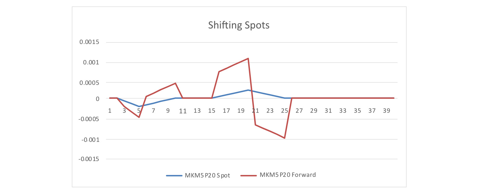
Below I will show that an in/decrease in the spot rate used for key rate calculation, does not produce in/decrease in forwards, nor does it preserve the pattern. Yet, an in/decrease in forwards produces in/decrease in the spots, albeit the pattern is not preserved due to the fact that spot rates are geometric means of forward rates. Note the wild patterns of forward rates when spot rates are shifted. However, a far smoother pattern of spots emerges when forwards are shifted. While the pattern by itself is not important, the expectation that an in/decrease in the rates should produce in/decrease in the underlying returns is important, and shifting spot rates does not provide that to the underlying forward rates used in the crediting rate.
Below is the impact of 10-bp up shifts to forward rates when spots are shifted.
Insert Figure A1.1 here
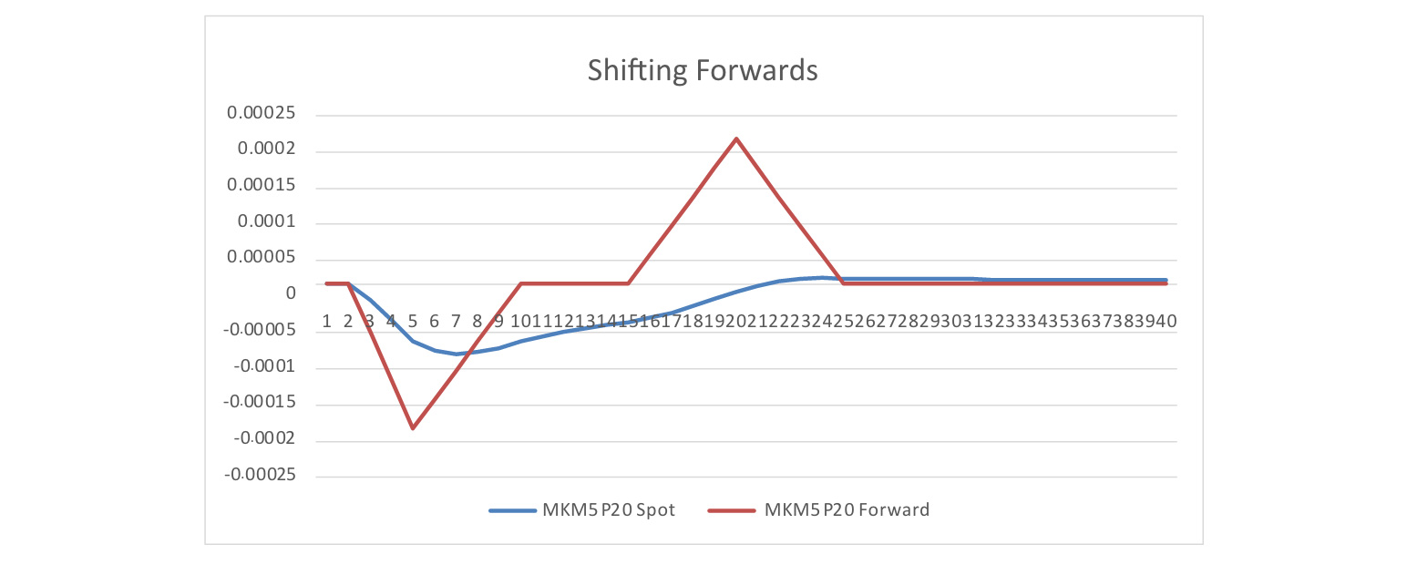
Below is the impact of 10-bp up shifts to spot rates when forwards are shifted.
Insert Figure A1.2 here
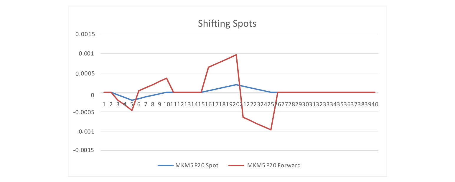
Below is the cross key-rate shift with a downshift to a five-year key rate and an upshift to a 20-year key rate using the shift to spot rates.
Insert Figure A1.3 here
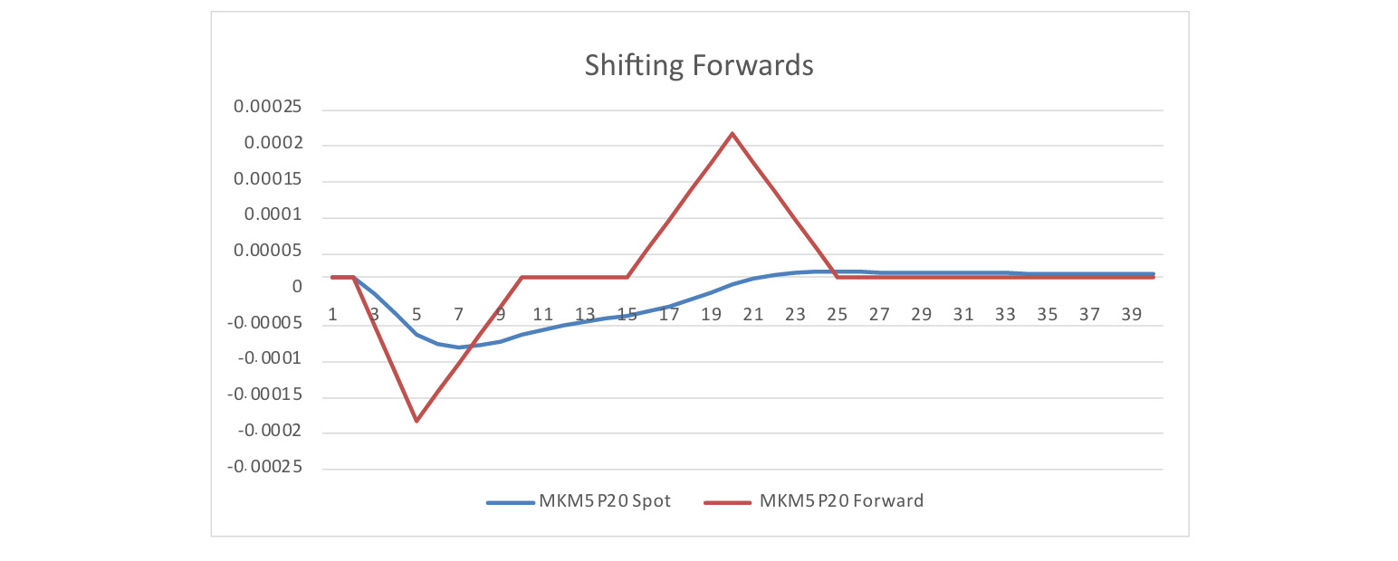
Below is the cross key-rate shift with a downshift to a five-year key rate and an upshift to a 20-year key rate using the shift to forward rates.
Insert Figure A1.4 here
Appendix 2
The tables below in Figure A2.1 compare Unscaled and Cumulative approaches using a shift to forward rate using both five key rates (two, five, 10, 20, and 30) and seven key rates (two, five, 10, 15, 20, 25, and 30). It can be seen that the cumulative approach produces results that are materially close to the unscaled approach and, in fact, at times outperforms it even though it uses 1/(number of key rates) of the runs. I did not see material deterioration of the approximation by decreasing the key rates from seven to five based on the simple product I had tested. I recommend testing five versus seven key rates for your portfolio and deciding if the reduction of four runs (two key rates combined with up and downshifts) would outweigh the possible level of less accuracy in the approximation for your portfolio.
Statements of fact and opinions expressed herein are those of the individual authors and are not necessarily those of the Society of Actuaries, the newsletter editors, or the respective authors’ employers.
Dariush Akhtari, FSA, FCIA, MAAA, is chief actuary at Converge RE. He can be contacted at dakhtari@converge-re.com.