Model Validation 101: Bring Your Calculus Mindset!

Validation is essential to the success of any model development process. Even for established models, results should be reviewed with a critical eye to ensure they make sense. Applying a calculus mindset can help ensure that your model works as expected. The validation process can also provide insights that help with the management of your business!

This article will focus on model validation in the context of reserve valuation, but these concepts have application in other branches of actuarial work, like pricing or risk management. With the inception of principle-based reserves or PBR (VM-20 for life, VM-21 for variable annuities and VM-22 for fixed annuities), modeling is now central to the US statutory valuation process. Modeling frameworks are also prevalent outside the US—e.g., Solvency II and Bermuda’s Economic Balance Sheet. Given the added complexity of these models, it is crucial for actuaries to have confidence in model results. Model validation helps to build that confidence.

Brief Calculus Refresher

Calculus has been used by life companies in the investment management process for decades to control asset–liability mismatch risk. Investment managers seek to minimize the volatility of surplus by matching the duration of assets and liabilities. Duration, or more specifically modified duration, is the first derivative with respect to yield of the unit value function for an asset or liability. Modified duration measures the slope of the value function–the rate of change in value per 1% change in yield. Matching the duration of assets and liabilities minimizes surplus fluctuations due to interest rates changes.

As a simple example of the modified duration calculation, consider a non-callable five-year zero coupon bond that pays $1 at maturity. The value of this bond is a function of the prevailing market yield rate i:

The first derivative of this function with respect to i is

To get modified duration, divide the first derivative by the value function:

The negative value of this expression indicates that the slope of the value function is negative–as interest rates increase, the value of the bond decreases. For i = 4%, the derivative is -5 / 1.04 = -4.81. This means that at the 4% yield point, each 1% increase/decrease in yield rate will decrease/increase the bond’s market value by approximately 4.81%.

Duration becomes more difficult to measure when value is a function of other variables like bond call options and policyholder behavior options, such as lapse and partial withdrawal for insurance and annuity contracts. That’s because options are more likely to be exercised when they are in-the-money. For example, the lapse rate of a deferred annuity contract crediting 4% interest increases as rates offered by competitors increase above 4%.[1] This difficulty is overcome by applying the concept of effective duration. Effective duration determines the slope of the asset or liability value function by calculating values at different yield rates—inclusive of option behavior assumptions—and using this information to derive the slope of the value curve. The formula for effective duration at yield rate i is:

where D is a small marginal change in the yield rate, such as 0.1%. The effective duration of our zero-coupon bond paying $1 at the end of five years is calculated at the 4% yield point as follows:

Value (3.9%) = 1 / 1.039^5 = 0.8259

Value (4.0%) = 1 / 1.040^5 = 0.8219

Value (4.1%) = 1 / 1.041^5 = 0.8180

Effective Duration (4.0%) = (0.8180 – 0.8259) / (0.8219 x 2 x 0.1%) = -4.81

The -4.81 effective duration matches the modified duration derived from calculus. While more work to determine than modified duration, effective duration enables calculation of slope for functions that don’t lend themselves to pure calculus, like PBR models that involve a lot of different variables.[2]

Application to Modeling

PBR models typically involve many different liability-related assumptions: Mortality, lapse, partial withdrawal, premium persistency, rider utilization, expense and possibly morbidity. These assumptions may reflect dynamic policyholder behavior that differs by economic scenario—e.g., withdrawal rates may increase with increasing interest rates, because policyholders may remove funds to reinvest outside the policy to obtain higher current yields.

The PBR approach differs from traditional reserving in that projected benefit and expense streams are not discounted at a single interest rate. Instead, the discount rate is a function of yields on assets held on the valuation date, assets acquired through reinvestment, and market gains or losses on assets sold before maturity to meet benefit obligations. In the PBR world, it is useful to think of the reserve as the statement value of assets needed on the valuation date to mature all obligations, using modeled assumptions. If the assets are exactly sufficient, the PBR projection will generate a surplus of $0 after the final benefit payment has been made.

Both VM-20 and VM-21 prescribe a direct iteration method (DIM) for calculating scenario reserves.[3] Under DIM, each projection starts with the initial asset portfolio that backs the specified liabilities. These assets may be either insufficient or more than sufficient to produce zero surplus at the end of each projection. An iterative process is then applied to solve for the additional assets (or asset reduction) needed to produce zero surplus at the end of each projection. The scenario reserve then equals the sum of the statement value of the initial asset portfolio plus (or minus) the additional assets (or asset reduction). Models built in Excel can use the Goal Seek function to perform the DIM.

Once a PBR model is developed, the actuary must validate the results.[4] We can use the calculus techniques described above to do an important part of the validation. A good test for all models is to run sensitivities to determine whether the model behaves as expected when small changes are made to assumptions and/or data. Measuring the impact of small changes is the essence of the calculus differentiation process!

A Simple Example

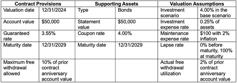
The following Excel model provides an example of sensitivity testing. We use a fixed-rate deferred annuity contract with these characteristics:

The model uses several simplifying assumptions:

• No death terminations prior to contract maturity, i.e., the mortality rate is zero. A full PBR model would apply mortality rates appropriate to the policyholder’s age in each year of the projection.
• No asset defaults. A full PBR model would apply default rates appropriate to the credit rating of each asset.
• All reinvested cash earns a single rate, and cash shortfalls are funded by borrowing at this rate. In the base scenario, the rate is 4%. A full PBR model would reflect reinvestment at different rates along the yield curve, selling assets to cover shortfalls, and fluctuations in the curve over the projection horizon.
• Annual time step. Full PBR models may use shorter time steps, such as monthly, to improve accuracy.

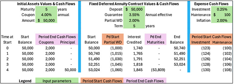
Table 1 below is a projection of values and cash flows for the initial asset portfolio, the annuity contract and expenses over the projected life of the contract.

Table 1
Fixed-Rate Deferred Annuity PBR Model – Projected Values

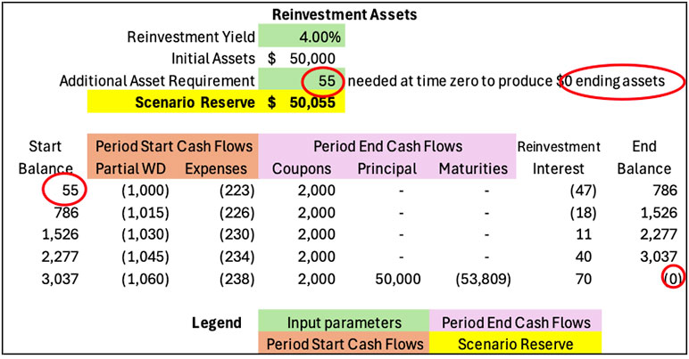
Table 2 below shows projected reinvestment activity and cumulative assets in the base (4%) scenario, using cash flows from Table 1 above.

Table 2
Fixed-Rate Deferred Annuity PBR Model – Base Scenario Reserve Valuation

In this scenario, the DIM implemented through Excel Goal Seek determined that the $50,000 initial asset portfolio must be augmented by $55 to produce $0 assets after the contract has matured. Since there is no remaining liability after maturity, surplus is also $0. Thus, the scenario reserve in this base case is $50,055.

Having established the base scenario, let’s sensitivity test using calculus and the concept of effective duration to validate that the model is working properly. The word “duration” is generally associated with measuring the sensitivity of asset or liability values to yield rate changes. Since the concept will be extended to sensitivities not related to yield, henceforth this metric will be called “slope” rather than “duration” to avoid confusion.

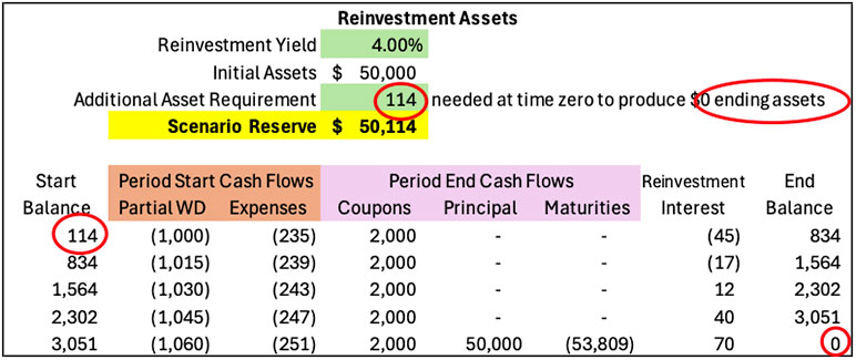
First, let’s see what happens if we increase the investment expense rate by 10%, from the base rate of 0.25% to 0.275%. Table 3 below shows the results of the reinvestment projection after applying the DIM.

Table 3
Fixed-Rate Deferred Annuity PBR Model – Alternative Scenario Reserve Valuation

As expected, expense cash flows increased but other cash flows—partial withdrawals, coupons, principal and maturities—did not. To achieve $0 ending assets, the DIM determined that $114 must be added at time zero, bringing the scenario reserve to $50,114—an increase of $59 from the base scenario. This seems intuitive: If expenses increase, more assets are needed at the start of the projection to mature obligations, which include both benefit payments and expenses incurred to administer the contract.

Now let’s decrease the investment expense rate by 10%, from 0.25% to 0.225%. The DIM solves for a scenario reserve of $49,996, which is $59 less than the base reserve. Having determined the scenario reserve at three points, we apply the effective duration formula to calculate the slope of the investment expense variable at the 0.25% point:

Slope = ($50,114 - $49,996) / (2 x 10% x 0.25% x $50,055) = 4.7

Thus, for each $1 added (or subtracted) from the annual investment expense requirement, there is a $4.70 increase (decrease) in the scenario reserve. This seems intuitive—the contract has a five-year life, so increasing expenses by $1 per year should increase the reserve roughly by the present value of $1 per year for five years. Thus, the model passes the validation test for the investment expense variable!

Table 4 below shows the slope calculations for this and several other sensitivities.

Table 4
Fixed-Rate Deferred Annuity PBR Model – Sensitivity Testing Results

• Partial Withdrawals: The base assumed rate is 2%. Sensitivity testing produces a slope of +0.03 which is close to zero. Why? Because each dollar withdrawn extinguishes part of the future maturity payment, so changing withdrawal rates doesn’t have much impact on total benefit payments.
• Bond Coupon: Now, change the starting asset portfolio to use bonds with coupon rates either higher or lower than in the base case. The slope of this assumption is -4.48, indicating that increasing the coupon by $1 reduces the scenario reserve by $4.48. This is similar to the impact of the investment expense assumption, but with opposite slope.
• Reinvestment Rate: Assuming initial investment in a five-year bond, the slope is -0.02, very close to zero. There is little impact because the bond cash inflows are well-matched to cash outflows from benefit payments and expenses, so there isn’t much reinvestment activity. If, however, the initial investment is a six-year bond, the slope increases to +0.78. In this case, the reinvestment rate becomes more impactful because at the end of five years, the bond must be sold one year prior to maturity to fund the contractual maturity payment. If the reinvestment rate has increased, the bond sale generates a capital loss, which diminishes assets, so a higher scenario reserve is required. This sensitivity highlights the importance of duration and cash flow matching to minimize investment-related risk.

After developing sensitivity testing capabilities, you can use them to validate results at the next reporting period. For example, if the market yield on reinvested assets increased during the period, you should be able to validate the impact of this change on the reserve.

Conclusion

This simple example shows how calculus concepts can be applied to measure and interpret the sensitivity of model results to changes in assumptions and data. Evaluate each sensitivity to determine whether it is intuitive. If the result is not intuitive, look for bugs in your model. But, if the result is intuitive, use it to educate colleagues about circumstances under which the modeled phenomenon can make or lose money for your organization. They will be impressed by your insights!

Statements of fact and opinions expressed herein are those of the individual authors and are not necessarily those of the Society of Actuaries, the newsletter editors, or the respective authors’ employers.